Casinos, gamble and Markov chains: Parrondo's Paradox!

So it’s not really any secret that casinos always have an edge over its customers. That is basically their business model: to always have the upper hand in their games such that, even if they lose sometimes, generally they win (even though this advantage doesn’t seem so meaninful in a way it would put away the gamblers).

The thing is, while this is relatively easy to achieve if you are careful enough to “isolate” your games in a way that they are unaffected by external variables, this is absolutely not the case otherwise!

A relatively popular example of this is Parrondo’s paradox. To start off, let’s toss some fair coins: if we get tails, we win one ticket. Otherwise we lose the same amount.

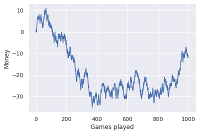
Sadly we lost at the end, even though the coin was fair (i.e. we had a \(50/50\) chance of winning). But had we kept trying, the end result would look something like this:

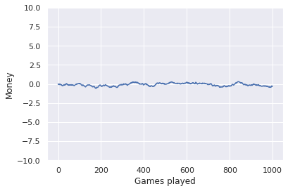
Tickets earned by games played averaged over \(1000\) games.

This is much smoother. And we can also see we are really winning and losing with the same frequency, since our balance barely leaves zero. Another way to look at it would be by playing a lot of games and plotting a histogram of the tickets earned at the end. In our case it would look something like this:

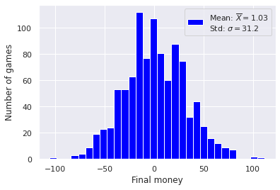
Histogram of tickets earned/lost after \(100\) fair coins tossed, done \(1000\) times.

If that looks like a Bell curve centered around zero, that’s because it is! And we can guarantee that with the central limit theorem.

Now consider a game just a little bit unfair, with a \(49.5\%\) chance of winnig, for example. Plottig the histogram in this case gives us the following:

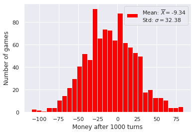
So it is still a Bell curve, however the mean is negative, which means we are losing more often than not (but that was expected).

Now imagine you are a bored casino owner thinking about new ways of making money and decide to create a brand new game. In order to trick the gamblers, you make the following rules:

- If the customer has a number of tickets that is a multiple of 3, he has a 9.5% chance of winning.

- However, if the number of tickets is not a multiple of 3, the chance of victory is 74.5%.

Would you play this game?

An average gambler, also trying to maximize its profits, might think something like this:

The first game is only played when my tickets are a multiple of \(3\), which means \(1\) out of \(3\) times I’ll only have a \(9.5\%\) probability of winning, while \(2\) out of \(3\) times I will be playing the good game. That means in the long run my chance of earning money is

\[\rho = \frac{1}{3} 0.095 + \frac{2}{3} 0.745 \approx 0.528\]

And while a fair line of thought, this is not exactly right, and the problem is with the assumption that the bad game is only played a third of the times. This is the part we dive into another rabbit hole.

Markov chains

So let’s move away from gambling for a while to talk about beans.

Imagine we have two different bean farmers conveniently named \(A\) and \(B\). Both their beans are great, but a person that buys from farmer \(A\) happens to have a \(20\%\) chance of buying from \(B\) next time (and therefore an \(80\%\) chance of buying from \(A\) again), while if you buy from \(B\), you have a \(60\%\) chance of buying from \(A\) next. This can be ilustrated graphically:

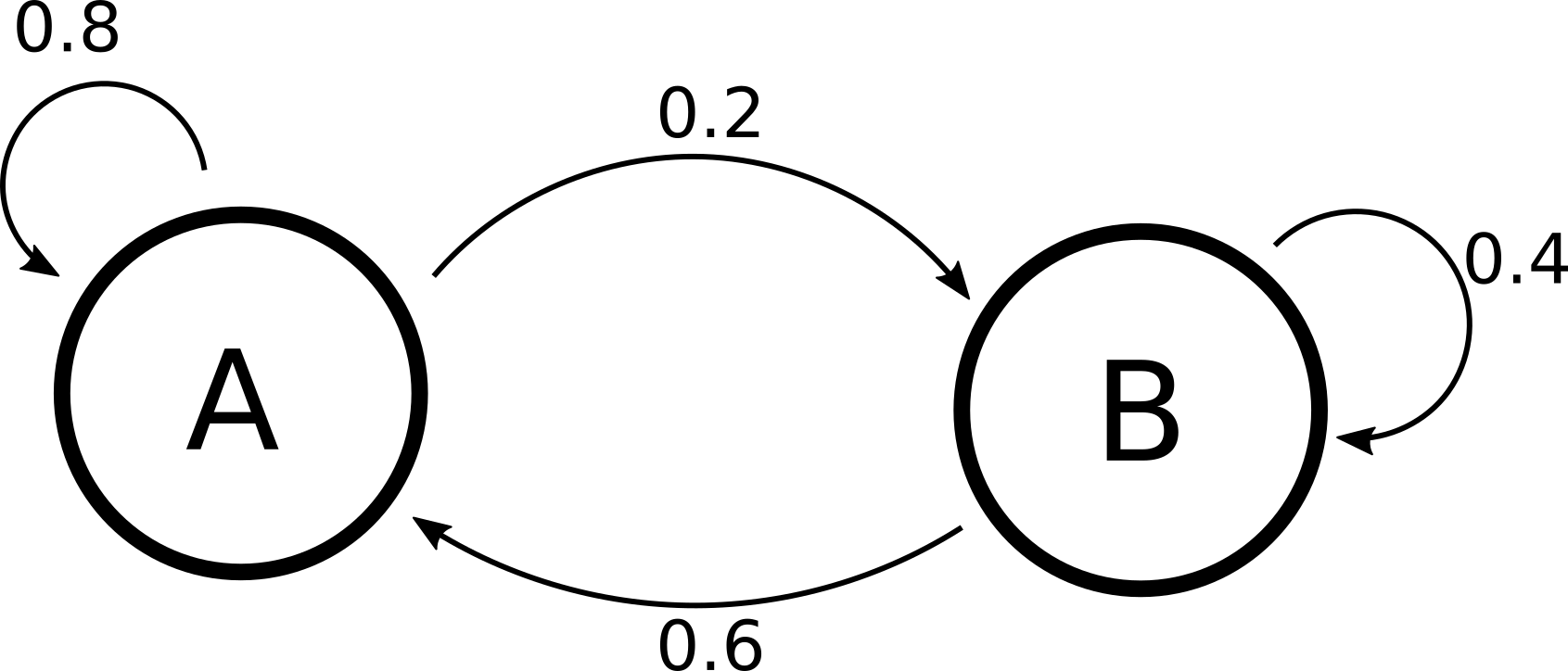
Or like this:

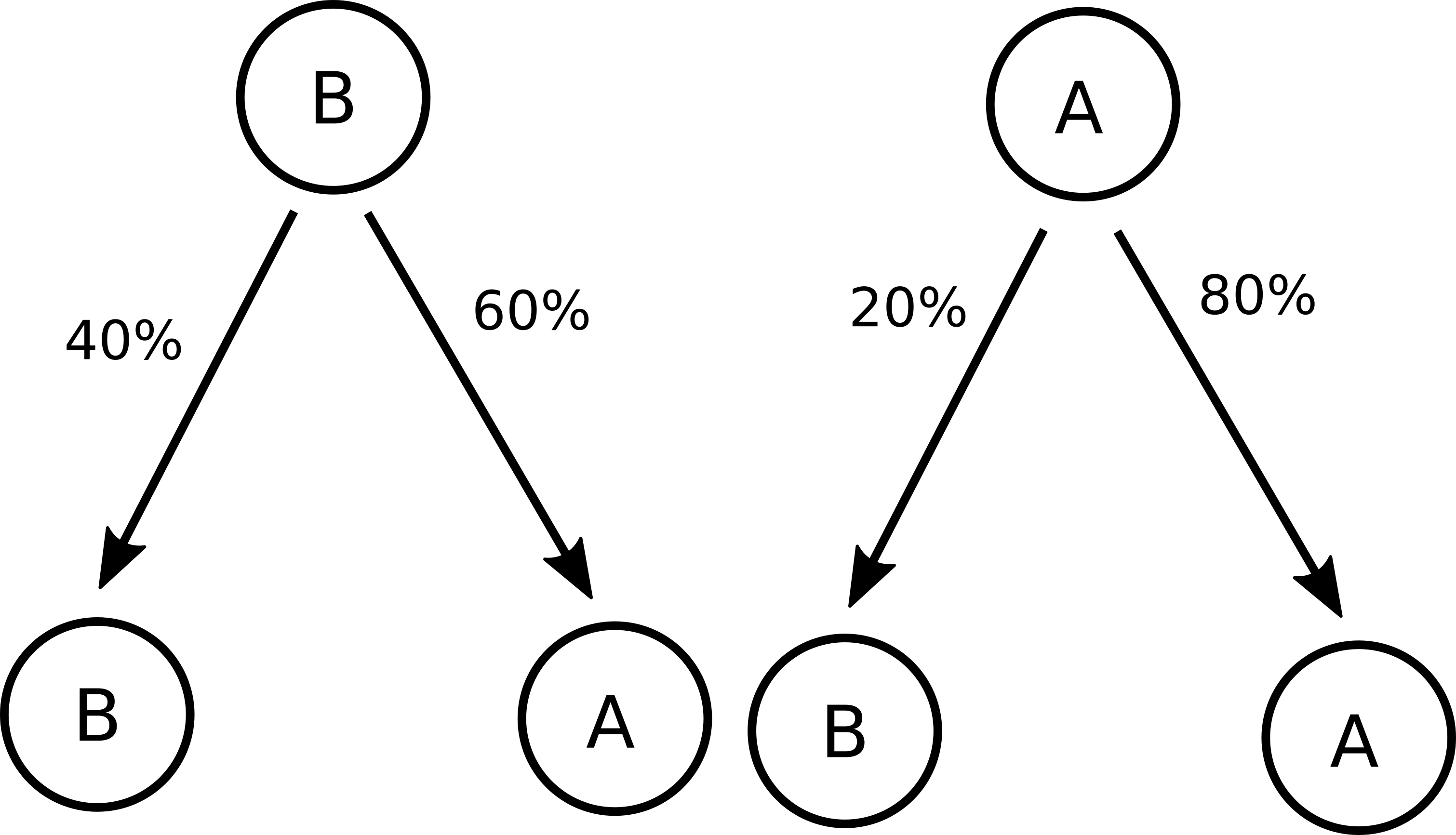
Question is: what happens? Suppose \(100\%\) of the population used to buy from \(A\) before \(B\) arrived, what percentage of it will start buying from \(B\) after a while? Would the end result be any different had we started with the customers equally divided between the two farmers? Let’s try visualizing that!

We start by defining the percentage of the population buying from \(A\) at any give time as \(S^{(A)}\), and from \(B\) as \(S^{(B)}\). Within one time step, the new values for the percentages will be given by:

as it consists of the new customers + the old customers that did not change bean farmers. We can write this as a matrix multiplication:

Now, if we wanted to get the result after two time steps, we could simply do:

and so on. The structure on which we are working here is called a Markov chain, and the square matrix with the probabilities is the stochastic matrix.

Enough of terminology, our goal here is to determine where this thing goes. Does \(S^{(A)}\) and \(S^{(B)}\) ever stabilize (that is, reach a fixed value) after a lot of timesteps? One way of checking this would be to start with some values for the \(S\)’s (keep in mind \(S^{(A)} + S^{(B)} = 1\) since we are talking about percentages) and just do this matrix multiplication over and over until a desired convergence. Another way of doing this would using the power of linear algebra.

The thing is, finding a fixed value for \(\textbf{S} = \left(\begin{array}{c} S^{(A)}\\ S^{(B)} \end{array}\right)\) means that

\(M\) being our stochastic matrix. Now, in linear algebra, if we have a vector space \(V\) over a field \(K\), given a linear transformations \(T : V \longrightarrow V\) (that is, it maps the vector space into itself), if we have a vector \(v \in V\) such that:

we call \(v\) an eigenvector of \(T\) with \(\lambda\) as its associated eigenvalue. In case you havent already, I would recomend watching this great video from 3Blue1Brown that explains this perfectly.

So, \(\textbf{S}\) is basically an eigenvector of our stochastic matrix with eigenvalue \(\lambda = 1\), and finding it (if we can) results on an exact solution for our problem. If all this seems unrigorous and a little bit hand-wavy, that’s because it is! Although we could develop the maths further if we wanted to, what we have here serves our purpose.

Now we are left with finding \(\textbf{S}\). If you try doing the matrix multiplications this will result on a linear system and our problem becomes a matter of solving it:

What gives us \(S^{(A)} = 0.75, S^{(B)} = 0.25\). That is, at the end it will settle for \(75\%\) of the population buying beans from \(A\) and \(25\%\) buying from \(B\). Indeed, let’s take a look at what would have happend had we chosen to calculate several timesteps:

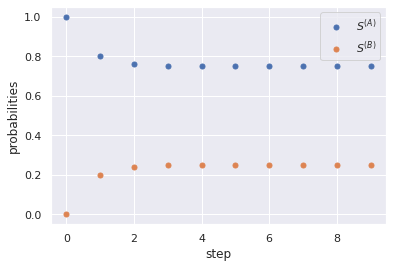
here we started with \(S^{(A)}_0 = 1, S^{(B)}_0 = 0\), but it does not really matter as the convergence radius inclues all possible scenarios

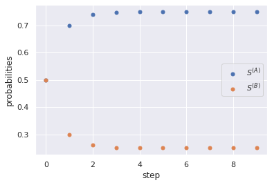
Now starting with \(S^{(A)}_0 = S^{(B)}_0 = 0.5\)

But what does this all have to do with our casino games? EVERYTHING!

Back to the game

Remember our second game, the one which we assumed had a one in three chance of having a bad winning probability. Now we do what is called a pro gamer move:

Divide our number of tickets in three possible sets: \(P^{(1)}, P^{(2)}\) and \(P^{(3)}\) like this:

These are our bean farmers, and we want to know what is, in the long run, the probability that we buy from each of those (i.e. what is the frequency we find ourselves in each set).

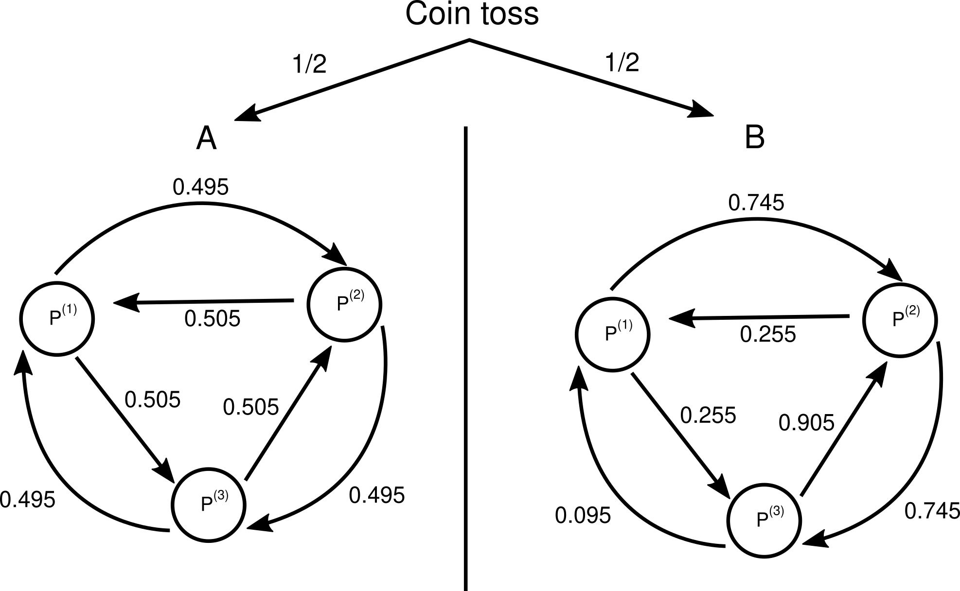
For that we use precisely the probabilities for winning in each case. For example, if we have a number of tickets equal \(3\), we belong to \(P^{(3)}\) and have a \(90.5\%\) chance of losing and dropping to \(2\) tickets, therefore changing to \(P^{(2)}\). Let’s graph this out:

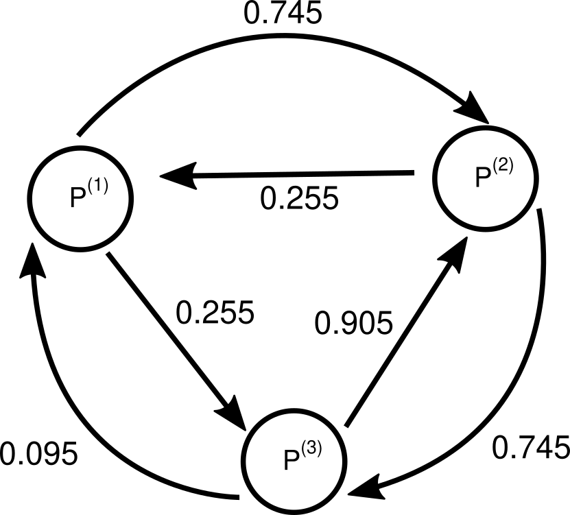
Now we write this down, defining the probabilities to have each amount of tickets as \(S^{(1)}, S^{(2)}\) and \(S^{(3)}\) for \(P^{(1)}, P^{(2)}\) and \(P^{(3)}\) respectivly:

As a matrix multiplication:

And we find the steady state (i.e. the eigenvector) \(\textbf{S} = \left(\begin{array}{c} \pi_{1}\\ \pi_{2}\\ \pi_{3} \end{array}\right)\)

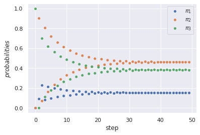
Convergence of the stochastic vector to the steady state over steps.

Solving it we end up with \(\pi_1 = 0.1543, \pi_2 = 0.4621\) and \(\pi_3 = 0.3836\). Notice it is indeed much different than the \(\frac{1}{3}\) we were expecting.

Now to get the overall probability of victory we simply multiply the chance of winning on each set \(P\) with the respective frequency we find ourselves in it. That is:

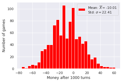
therefore leaving us with a \(49.56\%\) chance of success, which is still a disadvantage. We can also visualize this by playing this game multiple times and ploting the final number of tickets as a histogram:

Parrondo’s paradox starts here. What if, instead of playing those two games separately, each turn we tossed a coin to decide which game we were playing? Let’s plot the histogram for that.

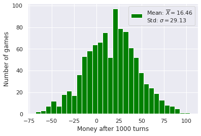
And suddenly we are winning! If we take the average number of tickets for each turn of these three cases (game \(A\), game \(B\) and games \(A\) and \(B\) randomly), we get the following:

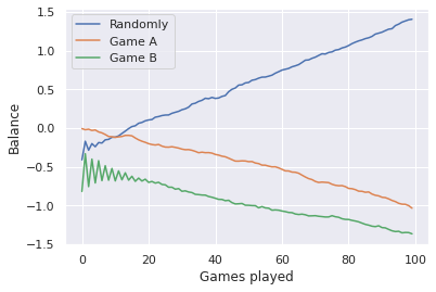
This seemingly paradoxical result was discussed on the Nature magazine’s article Losing strategies can win by Parrondo’s paradox by Gregory P. Harmer and Derek Abbott after its discovery by Juan Parrondo as published in Unsolved Problems of Noise and Fluctuations.

We already discussed all the required tools to describe mathematically what exactly is happening here. Let’s use our sets \(P^{(1)}, P^{(2)}\) and \(P^{(3)}\) deffined previously. Now, just like we did with game \(B\), think about game \(A\) in a similar fashion (even though the probabilities do not depend on the sets in this case). Consider the coin toss deciding which graph we will be working with and Dojyaaa~n!

Now we just include this when building our stochastic matrix:

sorry, mobile users.

Calculating the eigenvector for this matrix gives us \(\textbf{S} = \left(\begin{array}{c} 0.2541\\ 0.4008\\ 0.3451 \end{array}\right)\) and we once again calculate the overall winning probability:

which is a \(50.78\%\) chance of winning!

Now, we choose these numbers for illustration purposes, but the original paper states this should work for any sequences of games \(A\) and \(B\) (given a sufficient amount of iterations) and specific settings of probabilities for the games.

If you feel like experimenting with different parameters feel free to download this notebook. Also all the code and images used are avaliable here.

References

1. Gregory P. Harmer and Derek Abbott, Losing strategies can win by Parrondo’s paradox
2. Derek Abbot, Peter Taylor, and Juan Parrando, Parrondo’s Paradoxical Games and the Discrete Brownian Ratchet
3. Juan Parrondo, Unsolved Problems of Noise and Fluctuations